MR Protocols: Difference between revisions
imported>Knk Created page with "== '''Gradwarp''' == * By default, the scanner applies a correction for nonlinearities in the gradients, called gradwarp. Presumably, the correction will make your images more ..." |
|||
| (219 intermediate revisions by 11 users not shown) | |||
| Line 1: | Line 1: | ||
This page offers advice about how to set up your scan protocols and save the information. The wiki pages take you through the template protocols we think are most widely used. These protocols can be found on the the scanner console, saved under “CNI/head” within the protocol pool. | |||
Screenshots to remind you about how to set specific MRI protocols can be found on the page [[Setting up protocols page | Setting up protocols]] | |||
= | = General = | ||
* | == Setting up an MR scan protocol == | ||
A basic MR scan session usually starts with the following scans: | |||
* '''Localizer''' - a 3-plane localizer or 'scout' scan meant to find the subject's head. It is also be used for prescription for the subsequent scans. Doing some sort of localizer is necessary, and the '3planeloc SSFSE' (single shot fast spin echo) is the standard work-horse used by most CNI users. | |||
* '''Anatomical''' - usually a 3D T1-weighted scan at 0.9mm or 1mm isotropic resolution. It is essential for image alignment and anatomical analysis. More choices of anatomical scans are listed in the Anatomical imaging section. | |||
* | * '''ASSET calibration''' - a calibration scan for parallel imaging. It should be run before any scans that will use ASSET, such as GE's conventional fMRI and diffusion scans. | ||
* '''Higher-order shim''' - measures the magnetic field inhomogeneity and corrects it with polynomial gradients up to 2nd order. It should be run after ASSET and before fieldmap, fMRI or diffusion scans. | |||
* | * '''Field map''' - measures the magnetic field inhomogeneity that cannot be corrected by the shim and saves the inhomogeneity in a field map. It should be run immediately before or after the fMRI scan. | ||
At this point you will want to add a number of '''functional''' scans, '''diffusion''' scans or other type of scans based on your experiment. In the [[#MRI Protocol Templates | next section]] we describe templates for different categories of MRI protocols. The protocol templates are organized by category. One set is based on conventional multislice (2D) or 3D methods, a second set is based on the new simultaneous multislice (SMS) protocols (also called mux or multiband), and a third set are some special methods (spectroscopy and qMRI). | |||
You can get help in customizing the parameters from the CNI staff (ask Hua, Adam, or Laima). | |||
== ''' | == Saving your protocol parameters == | ||
=== Save screen-shots === | |||
At the GE console, you can save screen shots of the GE interface to show the main parameters that you have set in a protocol. Just get to the screen that you want to save, then press the 'Prnt Scrn' button on the keyboard. A little dialog will show up. You can choose to print, which will print on paper to the Laser printer in the control room. However, we strongly suggest that you save some trees and the toxic ink chemicals by saving a digital copy instead. To do this, type ina reasonable name in the filename field (default is 'screen') and hit the 'PNG" button. A PNG image will then magically appear in the 'screensaves' folder on the linux machine next to the console (cnirt). From there, you can email the images to yourself. Or, even better, create your own personal wiki page here that describes your protocol (just log in with your SUNet ID) and put the images in there. Then, you will always have them available when needed! THis is also a great way to share protocol information with your colleagues. | |||
=== Get a PDF of all protocol parameters === | |||
You can get a complete PDF of all your protocol info with a few clicks of the mouse. It's not quite as easy as a screensave, so we outline the procedure here. Note - There is a change on figure 4 - The pdf file will now appear with some viewing options at the top of the pdf file. By clicking on the 4th option from the right (a square with three parallel lines) the drop down menu will display a "save a copy" option which will result in the pdf being saved in the screensaves folder on the Linux machine (voxel2) next to the scanner. | |||
<gallery perrow=5> | |||
Image:Export_protocol_button.png|Click the "Protocol Exchange" button under the Image Management tab. | |||
Image:ExportMode.png|Select "Export Mode" and click OK in the dialog that comes up. | |||
Image:ProtocolSelection.png|Find your protocol in the next dialog, drag it to the "Protocol Selection" panel, and make sure it is selected. Then press the "preview" button. | |||
Image:SavePdf.png|You'll then see the PDF of your protocol. Right-click anywhere within the pdf and select "Save as..." from the drop-down menu. | |||
Image:SaveAs.png|Type the path and filename. Be sure that the path is /usr/g/mrraw/screensaves/ so it'll magically appear in the "screensaves" directory on the linux box. | |||
</gallery> | |||
== MRI protocol templates == | |||
The CNI has stored example protocols for anatomical, fMRI, diffusion, spectroscopy and quantitative MR scans (named as "CNI Examples", stored under "CNI / Head"). Depending on the user's needs, there are several ways to run a scan session. The stored protocols are meant to be used as a 'menu' from which you select the sequence that you want, based on your needs. While there are many variations stored there, here we just highlight a couple of the most common versions. A detailed list of all parameters for all scans can be found in the PDF files for each protocol. Some suggested ways of selecting from and set up these scans for your own scan session are described below. | |||
== Moving protocols from CNI to Lucas == | |||
If you plan to transfer scan protocols from the CNI to Lucas Center, please contact Hua and follow the steps below: | |||
* Let CNI staff know the (a) name of the protocol(s) to transfer and (b) which Lucas scanner. It would be useful if you could include a list of scans in your protocol too. We will help transfer the protocol files over to Lucas. | |||
* If your protocol contains pulse sequences provided by researchers outside CNI, then please let them know about the transfer so that they can prepare the sequences for you at Lucas. For example, if you run any spectroscopy sequences, then please let [mailto:mgu@stanford.edu Dr Meng Gu] know about the transfer plan. | |||
* Follow up with Lucas staff about setting up peripheral devices, e.g. response box, scanner trigger, visual display, physio recording, etc. The visual display at both Lucas scanners uses a projector and a screen mounted on the head coil. Another thing to keep in mind is that '''Lucas scanners do not send out scan triggers in the same way as the CNI scanner does''', so it’s preferred to let the stimulation program trigger the scanner by writing out a byte through the usb-serial port. Lucas also provides their version of the functional sequences that send out triggers to the computer, if you prefer to let the scanner trigger your stimulation. For more details please seek advice from the Lucas staff. | |||
The process | * The Lucas center has its own instance of Flywheel [http://lucascenter.flywheel.io lucascenter.flywheel.io]. '''Prior to scanning at Lucas, please be sure to coordinate with Tom Brosnan, or [mailto:lmperry@stanford.edu Michael Perry], to have your group’s accounts and projects configured.''' Michael can help you make sure your projects have the correct gear rules configured to process your data, which is an important consideration to maintain consistency across the two sites. As a good first approximation you can map existing project gear rules at CNI to your new projects at Lucas. Our goal is to make the same gears available at Lucas as are available at CNI. This is a work in progress. | ||
= Conventional imaging = | |||
== Anatomical imaging == | |||
===T1 weighted === | |||
All the suggested T1-weighted scans use GE's "BRAVO" sequence. It is an IR-prep, fast SPGR sequence with parameters tuned to optimize brain tissue contrast. Unless you have good reason to do so, you probably don't want to play with any parameters other than slice orientation, voxel size, and bandwidth. And for those, most users just pick one of the suggested configurations: | |||
* T1w 1mm ax (3:22): T1-weighted, 1mm^3 voxel size, 3D Bravo, axial slices. A single scan gives good signal-to-noise quality. If you just want a basic, fast, axial T1 weighted scan, go with this. | |||
* T1w 1mm sag (3:43): T1-weighted, 1mm^3 voxel size, 3D Bravo, sagittal slices. A single scan gives good signal-to-noise quality. This is similar to the 1mm axial, but with sagittal slice orientation. Compared to axial, this orientation is slightly less efficient because you need a full phase FOV, but sagittal slices usually do better than axial with artifacts from large blood vessels (e.g., carotid artifacts land in non-brain regions rather than the temporal lobes) and with fat-shift artifacts, because the shifted scalp signal usually misses the brain while with axial it can sometimes overlap the occipital lobe gray matter, causing tissue segmentation problems. | |||
* T1w 0.9mm sag (4:49) T1-weighted, 0.9mm^3 voxel size, 3D Bravo, sagittal slices. A single scan gives good signal-to-noise quality. As with the above scan, but a little higher spatial resolution. If you can afford to take 5 minutes for a T1 scan, this one is a great choice. This is our work-horse. Note: to get true .9 isotropic voxels, enter '23.04' for the FOV. The scanner GUI will display this as '23.0', but will store and use the full-precision that you type! | |||
* T1w 0.8mm sag (4:57 X 2): T1-weighted, 0.8mm^3 voxels, 3D Bravo, sagittal slices. Two scans (averaged in post-processing) are advised for good signal-to-noise quality. If you want to get better resolution, do two of these. | |||
* T1w 0.7mm sag (5:41 X 3): T1-weighted, 0.7mm^3 voxels, 3D Bravo, sagittal slices. 3-4 scans (averaged in post-processing) are advised for good signal-to-noise quality. If you can afford the time, and make use of high-quality anatomical images, this is the sequence to use. | |||
===T2 weighted === | |||
* 3D T2 (5:03): T2-weighted, 0.8mm^3 voxel size, 3D Cube T2, sagittal slices. A single scan gives good signal-to-noise quality. | |||
* 3D T2 FLAIR (6:17): T2-weighted, 1 mm^3 voxel size, 3D Cube T2, sagittal slices. An additional inversion-recovery pulse is applied in the 3D T2 CUBE sequence to suppress the CSF signal in the T2 weighted images. | |||
* 3D T2 PROMO (5:42): T2-weighted, 0.8mm^3 voxel size, 3D Cube T2, sagittal slices. PROMO (PROspective MOtion correction) adjusts the scan parameters during the scan to prospectively correct for patient motion and thus reducing the image artifacts. | |||
=== T2w/PDw === | |||
# | |||
2D T2w/PDw FSE (4:25): A standard 2D T2-weighted scan. You also get a bonus proton-density scan. Note that the two datasets will be interleaved; you'll want to separate them in post-processing. | |||
=== Technical Notes === | |||
In general, using a higher pixel bandwidth can help reduce chemical shift effects that push the fat signal from the scalp into the brain. | |||
The 3D Geometry Correction option uses a 3D correction for gradient non-linearity, over the 2D correction that is performed when the option is not checked. By including the slice direction in the correction, the resulting images are closer to geometric truth. The model used to represent gradient nonlinearity is the same as the 2D correction ("gradwarp") and it uses the same cubic interpolation function as the 2D correction. | |||
== Functional imaging == | |||
=== BOLD EPI (Full brain) === | |||
BOLD EPI 2.9mm 2sec: gradient echo EPI, 2.9mm^3 voxel size, 45 slices (~13 cm), TR/TE 2s/30ms, 2x in-plane acceleration. This sequence gives you full coverage of the brain. The 2x in-plane acceleration reduces the EPI distortion. This is a standard sequence for fMRI scans. | |||
=== BOLD EPI (High resolution, partial brain) === | |||
BOLD EPI 1.8mm 2sec (partial coverage): gradient echo EPI, 1.8mm^3 voxel size, 25 slices (~4.5 cm), TR/TE 2s/30ms, 2x in-plane acceleration. This sequence gives you partial coverage of the brain at a higher resolution. It is a good choice if you are interested in a particular part of the brain. | |||
===Technical Notes === | |||
If your protocol has multiple long-duration functional scans, you may consider doing additional field map measurements between the functional scans to access any field drift. See the [[Improving EPI]] page for information on fixing some common image problems with EPI images. | |||
There is a field map template protocol within the CNI/Head/CNI Example fMRI: Spiral fieldmap (0:27): 2D spiral, 1.75 x 1.75 x 2mm^3 voxel size. Copy the slice coverage of the BOLD scan. This scan generates a B0 field map in Hz (along with a magnitude image). | |||
The optimal echo time (TE) for BOLD fMRI at 3T is 30ms, where the difference in T2* decay of oxy/deoxy hemoglobin gives the highest contrast in the measured MR signals between the oxy/deoxy-genated blood. | |||
When doing BOLD fMRI, we prefer reading out the data at the optimal echo time quickly. When the TR (the repetition time) is shorter than the longitudinal relaxation time (T1) of the tissue of interest, we want to adjust the flip angle to optimize the SNR by maximizing the magnetization recovery along the z-axis (T1) during successive excitations of the same tissue. The optimal flip-angle is found by the Ernst equation: | |||
''flip-angle = acos(exp(-TR/T1)) '' | |||
[Note: this formula will return values in radians, which then need to be converted to degrees. Alternatively, if using Matlab, use the acosd function which will return degrees.] | |||
* A typical T1 value for gray matter is (3T): 1.33 seconds (Kruger, et al, 2001). (At 1.5T, it is closer to 0.9 seconds.) | |||
*Or use the following values for typical TRs at 3T: | |||
{|style="border-collapse: collapse; border-width: 1px; border-style: solid; border-color: #000" | |||
|- | |||
|style="border-style: solid; border-width: 1px; text-align: right"| '''TR (s):''' | |||
|style="border-style: solid; border-width: 1px; text-align: center"| 1 | |||
|style="border-style: solid; border-width: 1px; text-align: center"| 1.5 | |||
|style="border-style: solid; border-width: 1px; text-align: center"| 2 | |||
|style="border-style: solid; border-width: 1px; text-align: center"| 2.5 | |||
|style="border-style: solid; border-width: 1px; text-align: center"| 3 | |||
|style="border-style: solid; border-width: 1px; text-align: center"| 3.5 | |||
|style="border-style: solid; border-width: 1px; text-align: center"| 4 | |||
|style="border-style: solid; border-width: 1px; text-align: center"| 5 | |||
|style="border-style: solid; border-width: 1px; text-align: center"| 6 | |||
|style="border-style: solid; border-width: 1px; text-align: center"| 7 | |||
|- | |||
|style="border-style: solid; border-width: 1px; text-align: right"| '''flip (deg):''' | |||
|style="border-style: solid; border-width: 1px; text-align: center"| 61.9 | |||
|style="border-style: solid; border-width: 1px; text-align: center"| 71.1 | |||
|style="border-style: solid; border-width: 1px; text-align: center"| 77.2 | |||
|style="border-style: solid; border-width: 1px; text-align: center"| 81.2 | |||
|style="border-style: solid; border-width: 1px; text-align: center"| 84.0 | |||
|style="border-style: solid; border-width: 1px; text-align: center"| 85.9 | |||
|style="border-style: solid; border-width: 1px; text-align: center"| 87.2 | |||
|style="border-style: solid; border-width: 1px; text-align: center"| 88.7 | |||
|style="border-style: solid; border-width: 1px; text-align: center"| 89.4 | |||
|style="border-style: solid; border-width: 1px; text-align: center"| 89.7 | |||
|} | |||
== Diffusion weighted imaging == | |||
=== DTI === | |||
* DTI 2mm b1000 60dir (9:21): 2mm^2 voxel size, 60-70 axial slices, b-value 1000, 60 diffusion directions. | |||
=== HARDI === | |||
* DTI 2mm b2500 96dir (16:58): 2mm^2 voxel size, 60-70 axial slices, b-value 2500, 96 diffusion directions. | |||
If you are pressed for time, you can drop the b-value to 2000 and/or reduce the number of directions to 80: | |||
* DTI 2mm b2000 96dir (16:26): 2mm^2 voxel size, 60-70 axial slices, b-value 2000, 96 diffusion directions. | |||
* DTI 2mm b2000 80dir (12:37): 2mm^2 voxel size, 60-70 axial slices, b-value 2000, 80 diffusion directions. | |||
=== Technical Notes === | |||
Diffusion imaging at the CNI uses a modified version of GE's DW-EPI sequence. The sequence was modified so that for dual-spin-echo scans, the polarity of the second 180 degree pulse is inverted relative to the first 180. This causes off-resonance signal from fat to get defocused and thus help reduce fat-shift artifacts (See Sarlls et. al. Robust fat suppression at 3T in | |||
high-resolution diffusion-weighted single-shot echo-planar imaging of human brain. MRM 2011, PubMed PMID: [http://www.ncbi.nlm.nih.gov/pubmed/21604298 21604298] and Reese et. al. Reduction of eddy-current-induced distortion in diffusion MRI using a twice-refocused spin echo. MRM 2003, PubMed PMID: [http://www.ncbi.nlm.nih.gov/pubmed/12509835 12509835]). | |||
To decide on an optimal High Angular Resolution Diffusion Imaging (HARDI) acquisition protocol, see: | |||
* [http://www.ncbi.nlm.nih.gov/pubmed/19603409 White and Dale (2009)] Optimal diffusion MRI acquisition for fiber orientation density estimation: an analytic approach. HBM. (Calculated optimal b-values for maximum FOD estimation efficiency with SH expansion orders of L = 2, 4, 6, and 8 to be approximately b = 1,500, 3,000, 4,600, and 6,200 s/mm^2; demonstrated how scanner-specific hardware limitations generally lead to optimal b-values that are slightly lower than the ideal b-values.) | |||
* [http://www.ncbi.nlm.nih.gov/pubmed/18583153 Tournier et al. (2008)] Resolving crossing fibres using constrained spherical deconvolution: validation using diffusion-weighted imaging phantom data. NeuroImage. (For a 45 degrees crossing, the minimum b-value required to resolve the fibre orientations was ... 2000 s/mm^2 for CSD, and 1000 s/mm^2 for super-CSD.) | |||
* [http://www.ncbi.nlm.nih.gov/pubmed/17379540 Tournier et al. (2007)] Robust determination of the fibre orientation distribution in diffusion MRI: non-negativity constrained super-resolved spherical deconvolution. NeuroImage. | |||
HARDI data analysis tools include Camino, dipy, mrTrix etc. | |||
We use a modified version of the stock GE DWI-EPI pulse sequence. The resulting dicoms contain the diffusion parameters in these fields: | |||
* b-value (in sec/mm^2): 0043 1039 (GEMS_PARMS_01 block, item 1039) | |||
* gradient direction: [0019 10bb, 0019 10bc, 0019 10bd] (GEMS_ACQU_01 block, items 10bb - 10bd) | |||
In mrTrix (mapper.cpp), the following code is used to convert the dicom gradient values to the saved gradient directions: | |||
// M is the image transform | |||
M(0,0) = -image.orientation_x[0]; | |||
M(1,0) = -image.orientation_x[1]; | |||
M(2,0) = image.orientation_x[2]; | |||
M(0,1) = -image.orientation_y[0]; | |||
M(1,1) = -image.orientation_y[1]; | |||
M(2,1) = image.orientation_y[2]; | |||
M(0,2) = -image.orientation_z[0]; | |||
M(1,2) = -image.orientation_z[1]; | |||
M(2,2) = image.orientation_z[2]; | |||
M(0,3) = -image.position_vector[0]; | |||
M(1,3) = -image.position_vector[1]; | |||
M(2,3) = image.position_vector[2]; | |||
M(3,0) = 0.0; M(3,1) = 0.0; M(3,2) = 0.0; M(3,3) = 1.0; | |||
H.DW_scheme(s, 0) = M(0,0)*d[0] + M(0,1)*d[1] - M(0,2)*d[2]; | |||
H.DW_scheme(s, 1) = M(1,0)*d[0] + M(1,1)*d[1] - M(1,2)*d[2]; | |||
H.DW_scheme(s, 2) = M(2,0)*d[0] + M(2,1)*d[1] - M(2,2)*d[2]; | |||
If you get the data from the CNI Neurobiological Image Management System (NIMS), then the b-values and b-vectors have already been extracted for you and are provided along with the NIFTI file containing your data. These three files (the NIFTI, bvals, and bvecs files) can be send directly into most diffusion data analysis packages, such as the Stanford Vita Lab [[http://vistalab.stanford.edu/newlm/index.php/MrDiffusion mrDiffusion]] or FSL's [[http://www.fmrib.ox.ac.uk/fsl/fdt/index.html FDT]]. The b-values file contains a set of numbers (one for each acquired volume) that describe the b-value of the corresponding volume. The b-vecs file contains a triplet of numbers for each acquired volume, describing the diffusion-weighting direction for the corresponding volume. E.g., if you run our 60-direction scan, you will get 6 non-DW volumes followed by 60-DW volumes. Thus, you nifti file will contain 66 volumes. The b-vals file will contain 66 numbers (six 0's, fllowed by 60 1000's) and the b-vecs files will contain 66 triplets describing the DW directions for each volume (the triplets for the first 6 non-DW volumes are meaningless and can be ignored). | |||
=Simultaneous Multi-Slice (SMS)= | |||
The CNI, in collaboration with GE, implemented [http://www.sciencedirect.com/science/article/pii/S1090780713000311 simultaneous multi-slice EPI] (also known as multiband EPI). GE has integrated the SMS EPI into its product software platform, and since CNI's scanner upgrade to the UHP system, the SMS sequence is available as part of the GE product sequences, called the Hyperband. The Hyperband option is available for both BOLD EPI and diffusion EPI. | |||
Previously CNI has provided the SMS sequence using our research PSD, the one we referred to as the "mux" sequence. We recommend everyone who has been using the "mux" sequence to transition to the Hyperband sequence. For a comparison of features and performances between the "mux" and Hyperband sequence, please see this CNI blog [http://cni.stanford.edu/hyperband-transition/ Hyperband transition]. More information about the legacy "mux" sequence is described on the [[MUX EPI]] page. | |||
== SMS fMRI == | |||
The Hyperband sequence uses a calibration process that is integrated in the prescan. It is not necessary to set up a separate calibration scan or account for additional calibration volumes in the EPI time series. The calibration data is not saved in the final images. By default all the volumes in the EPI time series are reconstructed and saved in the final images, so the number of volumes in NIFTI is exactly the same amount as specified in the protocol (in the Multi-Phase page). However, the first few volumes in the time series may have different intensity because the spin magnetization has not yet reached steady state. In the BOLD analysis it may be necessary to discard the first few volumes in order to get to the steady state. Alternatively, there is an option in the Hyperband sequence to allow users to specify a number of dummy volumes, in which case the scanner will not reconstruct the first few volumes, but the scan timing is still the same, i.e. data acquisition starts right after the scan trigger. | |||
=== BOLD EPI === | |||
* Hyperband 6, voxel size 2.4mm^3, FOV 21.6cm, number of slices 60, TR 710ms (scan protocol in the Connectome project) | |||
* Hyperband 6, voxel size 1.8mm^3, FOV 23.0cm, number of slices 81, TR 1386ms | |||
* Hyperband 8, voxel size 3.0mm^3, FOV 22.2cm, number of slices 48, TR 415ms | |||
* Hyperband 8, voxel size 2.0mm^3, FOV 22.0cm, number of slices 72, TR 760ms | |||
=== Multi-echo EPI === | |||
* Hyperband 3, 2x in-plane acceleration, 3 EPI echoes, voxel size 2.8mm^3, FOV 22.4cm, number of slices 51, TR 1.49s, shortest TE 14.6ms, TE interval 23ms | |||
== SMS DWI == | |||
For SMS diffusion scans we generally recommend 2x to 3x slice acceleration, which will bring down the scan time by 2 to 3 times while maintaining the SNR of the diffusion weighted images. Partial Fourier acquisition is usually used to keep the TE as short as possible. The in-plane acceleration in addition to the slice acceleration is not always recommended because even though it can further reduce the EPI distortion but the SNR loss can be harmful for diffusion model fitting. | |||
Diffusion Spectrum Imaging (DSI) ([http://onlinelibrary.wiley.com/doi/10.1002/mrm.20642/full Magn. Reson. Med., 2005, 54: 1377–1386]) and multi-shell diffusion ([http://onlinelibrary.wiley.com/doi/10.1002/mrm.24736/full Magn. Reson. Med., 2013, 69: 1534–1540]) scans can be realized by designing gradient tables that specify direction and amplitude of the b-vectors. We set up a several customized gradient tables that are optimized for DTI, HARDI, 2 or 3-shell diffusion scans. Consult with us if you would like to set up your own diffusion gradient scheme. | |||
=== HARDI === | |||
* DTI 80dir 2mm (4:45): SMS factor 3, axial slices, 2mm^3 voxel size, number of slices 69, b-value 2500, 80 diffusion directions, 8 b=0 images | |||
* DTI 96dir 2mm (5:50): SMS factor 3, axial slices, 2mm^3 voxel size, number of slices 69, b-value 3000, 96 diffusion directions, 10 b=0 images | |||
=== Multi-shell diffusion === | |||
* DTI g79/81 b3k 2-shell (4:33+4:40): 2-shell with 10 b=0 images, 75 directions at b=1500, 75 directions at b=3000. SMS factor 4, voxel size 1.5mm^3, number of slices 84 (scan protocol in the Connectome project) | |||
* DTI g103 b2k 2-shell (4:50): 2-shell with 9 b=0 images, 30 directions at b=700, 64 directions at b=2000. SMS factor 3, 2x in-plane acceleration, voxel size 2mm^3, number of slices 75 | |||
* DTI g150 b3k 3-shell (6:15): 3-shell with 10 b=0 images, 30 direction at b=1000, 45 direction at b=2000, 65 direction at b=3000. SMS factor 3, 2x in-plane acceleration, voxel size 2mm^3, number of slices 63 | |||
= Scientific Protocols for Tissue and Chemistry = | |||
== Quantitative MR == | |||
These template protocols make quantitative measurements of MR parameters (e.g. T1 in seconds, and proton density (PD) as a fraction of the voxel) of brain tissue. Some 1 - PD is called the macromolecular tissue volume. | |||
=== T1 map === | |||
The SS-SMS T1 scan is a quantitative T1 scan using slice-shuffled inversion-recovery SMS EPI sequence. This scan gives you a T1 measurement at 2mm isotropic resolution in a minimum time. It uses in-plane acceleration therefore it's not necessary to run a separate pe1 scan for distortion correction unless you have enough time. For processing the NIFTI file from either pe0 or pe1 scan to get the T1 map, you can use [http://github.com/cni/t1fit/blob/master/t1_fitter.py this Python script]. If you acquired both pe0 and pe1, then you can use [http://github.com/cni/t1fit/blob/master/t1fit_unwarp.py this script] to process both NIFTI files to get the T1 map -- this includes an extra step for distortion correction using FSL's TOPUP before fitting the T1 relaxation. | |||
* SS-SMS T1 pe0 (pe1) (2:03): Gradient echo IR EPI, 2mm^3 voxel size, number of muxed slices 25 (75 unmuxed slices, 15cm), SMS factor 3, 2x in-plane acceleration, TR 3s. | |||
=== T1 map + PD map === | |||
The four SPGR scans, together with the four IR EPI scans, are set up for calculating T1 and PD maps using the [http://github.com/mezera/mrQ mrQ analysis package]. If you want a high resolution T1 map, or if you are interested in getting PD in addition to T1, then you should use this group of scans. | |||
* SPGR 1mm 30(4/10/20) deg (5:19 X 4): 3D SPGR, 1mm^3 voxel size, flip angle 30/4/10/20. The first scan should be run with Auto Prescan + Scan, and the following three should be run using Manual Prescan (do not change any parameters) + Scan. | |||
* IR EPI TI=50(400/1200/2400) (1:15 X 4): Gradient echo IR EPI, 1.875 x 1.875 x 4mm^3 voxel size, 2x in-plane acceleration. The first scan should be run with Auto Prescan + Scan, and the following three should be run using Manual Prescan (do not change any parameters) + Scan. | |||
Note that you could also choose to use only the four IR EPI scans to get a quantitative T1 map at a lower resolution. The working principle and model fitting procedure is explained [http://www-mrsrl.stanford.edu/~jbarral/t1map.html here]. | |||
== Spectroscopy == | |||
In-vivo spectroscopy sequences and analysis methods available and used at CNI are described [[GABA spectro | on this CNI spectroscopy page]]. | |||
= Additional information (deprecated) = | |||
== Device specific processing == | |||
The [[GE Processing | General Electric processing]] includes various steps that can influence the signal-to-noise of your data. We explain what we have learned about this and how to control it in the [[GE Processing]] page. | |||
== Technical notes == | |||
* [[media:bob_spatialRes_111216.pdf|Slides on spatial resolution]] from CNI tutorial | |||
* [[MR Signal Equations]] | |||
== Session Running Script == | |||
We advise you to put together a session running script that outlines set up of the scanner and peripherals and positioning of and communications with the participant. You can find an example [[media:Session_Running_Script.pdf|here]] (courtesy of Nanna Notthoff, Carstensen Lab). | |||
== CNI's Quality Assurance protocol == | |||
Weekly QA scans include: | |||
# BOLD EPI sequence (analyze mean and variance over time) | |||
# DW EPI sequence (analyze eddy current distortion stability) | |||
# Spiral field map (analyze long-term B0 stability) | |||
All QA scans are done on the fBIRN agar phantom. The phantom is positioned in the same orientation with the same padding each week. The landmark must be set to the same. The Rx should be not touched (use the same stored Rx). We should do HO shim and set the shim VOI to exactly cover the sphere. | |||
Latest revision as of 17:35, 23 August 2023
This page offers advice about how to set up your scan protocols and save the information. The wiki pages take you through the template protocols we think are most widely used. These protocols can be found on the the scanner console, saved under “CNI/head” within the protocol pool.
Screenshots to remind you about how to set specific MRI protocols can be found on the page Setting up protocols
General
Setting up an MR scan protocol
A basic MR scan session usually starts with the following scans:
- Localizer - a 3-plane localizer or 'scout' scan meant to find the subject's head. It is also be used for prescription for the subsequent scans. Doing some sort of localizer is necessary, and the '3planeloc SSFSE' (single shot fast spin echo) is the standard work-horse used by most CNI users.
- Anatomical - usually a 3D T1-weighted scan at 0.9mm or 1mm isotropic resolution. It is essential for image alignment and anatomical analysis. More choices of anatomical scans are listed in the Anatomical imaging section.
- ASSET calibration - a calibration scan for parallel imaging. It should be run before any scans that will use ASSET, such as GE's conventional fMRI and diffusion scans.
- Higher-order shim - measures the magnetic field inhomogeneity and corrects it with polynomial gradients up to 2nd order. It should be run after ASSET and before fieldmap, fMRI or diffusion scans.
- Field map - measures the magnetic field inhomogeneity that cannot be corrected by the shim and saves the inhomogeneity in a field map. It should be run immediately before or after the fMRI scan.
At this point you will want to add a number of functional scans, diffusion scans or other type of scans based on your experiment. In the next section we describe templates for different categories of MRI protocols. The protocol templates are organized by category. One set is based on conventional multislice (2D) or 3D methods, a second set is based on the new simultaneous multislice (SMS) protocols (also called mux or multiband), and a third set are some special methods (spectroscopy and qMRI).
You can get help in customizing the parameters from the CNI staff (ask Hua, Adam, or Laima).
Saving your protocol parameters
Save screen-shots
At the GE console, you can save screen shots of the GE interface to show the main parameters that you have set in a protocol. Just get to the screen that you want to save, then press the 'Prnt Scrn' button on the keyboard. A little dialog will show up. You can choose to print, which will print on paper to the Laser printer in the control room. However, we strongly suggest that you save some trees and the toxic ink chemicals by saving a digital copy instead. To do this, type ina reasonable name in the filename field (default is 'screen') and hit the 'PNG" button. A PNG image will then magically appear in the 'screensaves' folder on the linux machine next to the console (cnirt). From there, you can email the images to yourself. Or, even better, create your own personal wiki page here that describes your protocol (just log in with your SUNet ID) and put the images in there. Then, you will always have them available when needed! THis is also a great way to share protocol information with your colleagues.
Get a PDF of all protocol parameters
You can get a complete PDF of all your protocol info with a few clicks of the mouse. It's not quite as easy as a screensave, so we outline the procedure here. Note - There is a change on figure 4 - The pdf file will now appear with some viewing options at the top of the pdf file. By clicking on the 4th option from the right (a square with three parallel lines) the drop down menu will display a "save a copy" option which will result in the pdf being saved in the screensaves folder on the Linux machine (voxel2) next to the scanner.
-
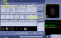 Click the "Protocol Exchange" button under the Image Management tab.
 -
 Select "Export Mode" and click OK in the dialog that comes up.
 -
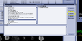 Find your protocol in the next dialog, drag it to the "Protocol Selection" panel, and make sure it is selected. Then press the "preview" button.
 -
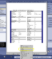 You'll then see the PDF of your protocol. Right-click anywhere within the pdf and select "Save as..." from the drop-down menu.
 -
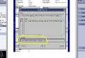 Type the path and filename. Be sure that the path is /usr/g/mrraw/screensaves/ so it'll magically appear in the "screensaves" directory on the linux box.


MRI protocol templates
The CNI has stored example protocols for anatomical, fMRI, diffusion, spectroscopy and quantitative MR scans (named as "CNI Examples", stored under "CNI / Head"). Depending on the user's needs, there are several ways to run a scan session. The stored protocols are meant to be used as a 'menu' from which you select the sequence that you want, based on your needs. While there are many variations stored there, here we just highlight a couple of the most common versions. A detailed list of all parameters for all scans can be found in the PDF files for each protocol. Some suggested ways of selecting from and set up these scans for your own scan session are described below.
Moving protocols from CNI to Lucas
If you plan to transfer scan protocols from the CNI to Lucas Center, please contact Hua and follow the steps below:
- Let CNI staff know the (a) name of the protocol(s) to transfer and (b) which Lucas scanner. It would be useful if you could include a list of scans in your protocol too. We will help transfer the protocol files over to Lucas.
- If your protocol contains pulse sequences provided by researchers outside CNI, then please let them know about the transfer so that they can prepare the sequences for you at Lucas. For example, if you run any spectroscopy sequences, then please let Dr Meng Gu know about the transfer plan.
- Follow up with Lucas staff about setting up peripheral devices, e.g. response box, scanner trigger, visual display, physio recording, etc. The visual display at both Lucas scanners uses a projector and a screen mounted on the head coil. Another thing to keep in mind is that Lucas scanners do not send out scan triggers in the same way as the CNI scanner does, so it’s preferred to let the stimulation program trigger the scanner by writing out a byte through the usb-serial port. Lucas also provides their version of the functional sequences that send out triggers to the computer, if you prefer to let the scanner trigger your stimulation. For more details please seek advice from the Lucas staff.
- The Lucas center has its own instance of Flywheel lucascenter.flywheel.io. Prior to scanning at Lucas, please be sure to coordinate with Tom Brosnan, or Michael Perry, to have your group’s accounts and projects configured. Michael can help you make sure your projects have the correct gear rules configured to process your data, which is an important consideration to maintain consistency across the two sites. As a good first approximation you can map existing project gear rules at CNI to your new projects at Lucas. Our goal is to make the same gears available at Lucas as are available at CNI. This is a work in progress.
Conventional imaging
Anatomical imaging
T1 weighted
All the suggested T1-weighted scans use GE's "BRAVO" sequence. It is an IR-prep, fast SPGR sequence with parameters tuned to optimize brain tissue contrast. Unless you have good reason to do so, you probably don't want to play with any parameters other than slice orientation, voxel size, and bandwidth. And for those, most users just pick one of the suggested configurations:
- T1w 1mm ax (3:22): T1-weighted, 1mm^3 voxel size, 3D Bravo, axial slices. A single scan gives good signal-to-noise quality. If you just want a basic, fast, axial T1 weighted scan, go with this.
- T1w 1mm sag (3:43): T1-weighted, 1mm^3 voxel size, 3D Bravo, sagittal slices. A single scan gives good signal-to-noise quality. This is similar to the 1mm axial, but with sagittal slice orientation. Compared to axial, this orientation is slightly less efficient because you need a full phase FOV, but sagittal slices usually do better than axial with artifacts from large blood vessels (e.g., carotid artifacts land in non-brain regions rather than the temporal lobes) and with fat-shift artifacts, because the shifted scalp signal usually misses the brain while with axial it can sometimes overlap the occipital lobe gray matter, causing tissue segmentation problems.
- T1w 0.9mm sag (4:49) T1-weighted, 0.9mm^3 voxel size, 3D Bravo, sagittal slices. A single scan gives good signal-to-noise quality. As with the above scan, but a little higher spatial resolution. If you can afford to take 5 minutes for a T1 scan, this one is a great choice. This is our work-horse. Note: to get true .9 isotropic voxels, enter '23.04' for the FOV. The scanner GUI will display this as '23.0', but will store and use the full-precision that you type!
- T1w 0.8mm sag (4:57 X 2): T1-weighted, 0.8mm^3 voxels, 3D Bravo, sagittal slices. Two scans (averaged in post-processing) are advised for good signal-to-noise quality. If you want to get better resolution, do two of these.
- T1w 0.7mm sag (5:41 X 3): T1-weighted, 0.7mm^3 voxels, 3D Bravo, sagittal slices. 3-4 scans (averaged in post-processing) are advised for good signal-to-noise quality. If you can afford the time, and make use of high-quality anatomical images, this is the sequence to use.
T2 weighted
- 3D T2 (5:03): T2-weighted, 0.8mm^3 voxel size, 3D Cube T2, sagittal slices. A single scan gives good signal-to-noise quality.
- 3D T2 FLAIR (6:17): T2-weighted, 1 mm^3 voxel size, 3D Cube T2, sagittal slices. An additional inversion-recovery pulse is applied in the 3D T2 CUBE sequence to suppress the CSF signal in the T2 weighted images.
- 3D T2 PROMO (5:42): T2-weighted, 0.8mm^3 voxel size, 3D Cube T2, sagittal slices. PROMO (PROspective MOtion correction) adjusts the scan parameters during the scan to prospectively correct for patient motion and thus reducing the image artifacts.
T2w/PDw
2D T2w/PDw FSE (4:25): A standard 2D T2-weighted scan. You also get a bonus proton-density scan. Note that the two datasets will be interleaved; you'll want to separate them in post-processing.
Technical Notes
In general, using a higher pixel bandwidth can help reduce chemical shift effects that push the fat signal from the scalp into the brain.
The 3D Geometry Correction option uses a 3D correction for gradient non-linearity, over the 2D correction that is performed when the option is not checked. By including the slice direction in the correction, the resulting images are closer to geometric truth. The model used to represent gradient nonlinearity is the same as the 2D correction ("gradwarp") and it uses the same cubic interpolation function as the 2D correction.
Functional imaging
BOLD EPI (Full brain)
BOLD EPI 2.9mm 2sec: gradient echo EPI, 2.9mm^3 voxel size, 45 slices (~13 cm), TR/TE 2s/30ms, 2x in-plane acceleration. This sequence gives you full coverage of the brain. The 2x in-plane acceleration reduces the EPI distortion. This is a standard sequence for fMRI scans.
BOLD EPI (High resolution, partial brain)
BOLD EPI 1.8mm 2sec (partial coverage): gradient echo EPI, 1.8mm^3 voxel size, 25 slices (~4.5 cm), TR/TE 2s/30ms, 2x in-plane acceleration. This sequence gives you partial coverage of the brain at a higher resolution. It is a good choice if you are interested in a particular part of the brain.
Technical Notes
If your protocol has multiple long-duration functional scans, you may consider doing additional field map measurements between the functional scans to access any field drift. See the Improving EPI page for information on fixing some common image problems with EPI images.
There is a field map template protocol within the CNI/Head/CNI Example fMRI: Spiral fieldmap (0:27): 2D spiral, 1.75 x 1.75 x 2mm^3 voxel size. Copy the slice coverage of the BOLD scan. This scan generates a B0 field map in Hz (along with a magnitude image).
The optimal echo time (TE) for BOLD fMRI at 3T is 30ms, where the difference in T2* decay of oxy/deoxy hemoglobin gives the highest contrast in the measured MR signals between the oxy/deoxy-genated blood.
When doing BOLD fMRI, we prefer reading out the data at the optimal echo time quickly. When the TR (the repetition time) is shorter than the longitudinal relaxation time (T1) of the tissue of interest, we want to adjust the flip angle to optimize the SNR by maximizing the magnetization recovery along the z-axis (T1) during successive excitations of the same tissue. The optimal flip-angle is found by the Ernst equation:
flip-angle = acos(exp(-TR/T1))
[Note: this formula will return values in radians, which then need to be converted to degrees. Alternatively, if using Matlab, use the acosd function which will return degrees.]
- A typical T1 value for gray matter is (3T): 1.33 seconds (Kruger, et al, 2001). (At 1.5T, it is closer to 0.9 seconds.)
- Or use the following values for typical TRs at 3T:
| TR (s): | 1 | 1.5 | 2 | 2.5 | 3 | 3.5 | 4 | 5 | 6 | 7 |
| flip (deg): | 61.9 | 71.1 | 77.2 | 81.2 | 84.0 | 85.9 | 87.2 | 88.7 | 89.4 | 89.7 |
Diffusion weighted imaging
DTI
- DTI 2mm b1000 60dir (9:21): 2mm^2 voxel size, 60-70 axial slices, b-value 1000, 60 diffusion directions.
HARDI
- DTI 2mm b2500 96dir (16:58): 2mm^2 voxel size, 60-70 axial slices, b-value 2500, 96 diffusion directions.
If you are pressed for time, you can drop the b-value to 2000 and/or reduce the number of directions to 80:
- DTI 2mm b2000 96dir (16:26): 2mm^2 voxel size, 60-70 axial slices, b-value 2000, 96 diffusion directions.
- DTI 2mm b2000 80dir (12:37): 2mm^2 voxel size, 60-70 axial slices, b-value 2000, 80 diffusion directions.
Technical Notes
Diffusion imaging at the CNI uses a modified version of GE's DW-EPI sequence. The sequence was modified so that for dual-spin-echo scans, the polarity of the second 180 degree pulse is inverted relative to the first 180. This causes off-resonance signal from fat to get defocused and thus help reduce fat-shift artifacts (See Sarlls et. al. Robust fat suppression at 3T in high-resolution diffusion-weighted single-shot echo-planar imaging of human brain. MRM 2011, PubMed PMID: 21604298 and Reese et. al. Reduction of eddy-current-induced distortion in diffusion MRI using a twice-refocused spin echo. MRM 2003, PubMed PMID: 12509835).
To decide on an optimal High Angular Resolution Diffusion Imaging (HARDI) acquisition protocol, see:
- White and Dale (2009) Optimal diffusion MRI acquisition for fiber orientation density estimation: an analytic approach. HBM. (Calculated optimal b-values for maximum FOD estimation efficiency with SH expansion orders of L = 2, 4, 6, and 8 to be approximately b = 1,500, 3,000, 4,600, and 6,200 s/mm^2; demonstrated how scanner-specific hardware limitations generally lead to optimal b-values that are slightly lower than the ideal b-values.)
- Tournier et al. (2008) Resolving crossing fibres using constrained spherical deconvolution: validation using diffusion-weighted imaging phantom data. NeuroImage. (For a 45 degrees crossing, the minimum b-value required to resolve the fibre orientations was ... 2000 s/mm^2 for CSD, and 1000 s/mm^2 for super-CSD.)
- Tournier et al. (2007) Robust determination of the fibre orientation distribution in diffusion MRI: non-negativity constrained super-resolved spherical deconvolution. NeuroImage.
HARDI data analysis tools include Camino, dipy, mrTrix etc.
We use a modified version of the stock GE DWI-EPI pulse sequence. The resulting dicoms contain the diffusion parameters in these fields:
- b-value (in sec/mm^2): 0043 1039 (GEMS_PARMS_01 block, item 1039)
- gradient direction: [0019 10bb, 0019 10bc, 0019 10bd] (GEMS_ACQU_01 block, items 10bb - 10bd)
In mrTrix (mapper.cpp), the following code is used to convert the dicom gradient values to the saved gradient directions:
// M is the image transform
M(0,0) = -image.orientation_x[0];
M(1,0) = -image.orientation_x[1];
M(2,0) =  image.orientation_x[2];
M(0,1) = -image.orientation_y[0];
M(1,1) = -image.orientation_y[1];
M(2,1) =  image.orientation_y[2];
M(0,2) = -image.orientation_z[0];
M(1,2) = -image.orientation_z[1];
M(2,2) =  image.orientation_z[2];
M(0,3) = -image.position_vector[0];
M(1,3) = -image.position_vector[1];
M(2,3) =  image.position_vector[2];
M(3,0) = 0.0; M(3,1) = 0.0; M(3,2) = 0.0; M(3,3) = 1.0;
H.DW_scheme(s, 0) = M(0,0)*d[0] + M(0,1)*d[1] - M(0,2)*d[2];
H.DW_scheme(s, 1) = M(1,0)*d[0] + M(1,1)*d[1] - M(1,2)*d[2];
H.DW_scheme(s, 2) = M(2,0)*d[0] + M(2,1)*d[1] - M(2,2)*d[2];
If you get the data from the CNI Neurobiological Image Management System (NIMS), then the b-values and b-vectors have already been extracted for you and are provided along with the NIFTI file containing your data. These three files (the NIFTI, bvals, and bvecs files) can be send directly into most diffusion data analysis packages, such as the Stanford Vita Lab [mrDiffusion] or FSL's [FDT]. The b-values file contains a set of numbers (one for each acquired volume) that describe the b-value of the corresponding volume. The b-vecs file contains a triplet of numbers for each acquired volume, describing the diffusion-weighting direction for the corresponding volume. E.g., if you run our 60-direction scan, you will get 6 non-DW volumes followed by 60-DW volumes. Thus, you nifti file will contain 66 volumes. The b-vals file will contain 66 numbers (six 0's, fllowed by 60 1000's) and the b-vecs files will contain 66 triplets describing the DW directions for each volume (the triplets for the first 6 non-DW volumes are meaningless and can be ignored).
Simultaneous Multi-Slice (SMS)
The CNI, in collaboration with GE, implemented simultaneous multi-slice EPI (also known as multiband EPI). GE has integrated the SMS EPI into its product software platform, and since CNI's scanner upgrade to the UHP system, the SMS sequence is available as part of the GE product sequences, called the Hyperband. The Hyperband option is available for both BOLD EPI and diffusion EPI.
Previously CNI has provided the SMS sequence using our research PSD, the one we referred to as the "mux" sequence. We recommend everyone who has been using the "mux" sequence to transition to the Hyperband sequence. For a comparison of features and performances between the "mux" and Hyperband sequence, please see this CNI blog Hyperband transition. More information about the legacy "mux" sequence is described on the MUX EPI page.
SMS fMRI
The Hyperband sequence uses a calibration process that is integrated in the prescan. It is not necessary to set up a separate calibration scan or account for additional calibration volumes in the EPI time series. The calibration data is not saved in the final images. By default all the volumes in the EPI time series are reconstructed and saved in the final images, so the number of volumes in NIFTI is exactly the same amount as specified in the protocol (in the Multi-Phase page). However, the first few volumes in the time series may have different intensity because the spin magnetization has not yet reached steady state. In the BOLD analysis it may be necessary to discard the first few volumes in order to get to the steady state. Alternatively, there is an option in the Hyperband sequence to allow users to specify a number of dummy volumes, in which case the scanner will not reconstruct the first few volumes, but the scan timing is still the same, i.e. data acquisition starts right after the scan trigger.
BOLD EPI
- Hyperband 6, voxel size 2.4mm^3, FOV 21.6cm, number of slices 60, TR 710ms (scan protocol in the Connectome project)
- Hyperband 6, voxel size 1.8mm^3, FOV 23.0cm, number of slices 81, TR 1386ms
- Hyperband 8, voxel size 3.0mm^3, FOV 22.2cm, number of slices 48, TR 415ms
- Hyperband 8, voxel size 2.0mm^3, FOV 22.0cm, number of slices 72, TR 760ms
Multi-echo EPI
- Hyperband 3, 2x in-plane acceleration, 3 EPI echoes, voxel size 2.8mm^3, FOV 22.4cm, number of slices 51, TR 1.49s, shortest TE 14.6ms, TE interval 23ms
SMS DWI
For SMS diffusion scans we generally recommend 2x to 3x slice acceleration, which will bring down the scan time by 2 to 3 times while maintaining the SNR of the diffusion weighted images. Partial Fourier acquisition is usually used to keep the TE as short as possible. The in-plane acceleration in addition to the slice acceleration is not always recommended because even though it can further reduce the EPI distortion but the SNR loss can be harmful for diffusion model fitting.
Diffusion Spectrum Imaging (DSI) (Magn. Reson. Med., 2005, 54: 1377–1386) and multi-shell diffusion (Magn. Reson. Med., 2013, 69: 1534–1540) scans can be realized by designing gradient tables that specify direction and amplitude of the b-vectors. We set up a several customized gradient tables that are optimized for DTI, HARDI, 2 or 3-shell diffusion scans. Consult with us if you would like to set up your own diffusion gradient scheme.
HARDI
- DTI 80dir 2mm (4:45): SMS factor 3, axial slices, 2mm^3 voxel size, number of slices 69, b-value 2500, 80 diffusion directions, 8 b=0 images
- DTI 96dir 2mm (5:50): SMS factor 3, axial slices, 2mm^3 voxel size, number of slices 69, b-value 3000, 96 diffusion directions, 10 b=0 images
Multi-shell diffusion
- DTI g79/81 b3k 2-shell (4:33+4:40): 2-shell with 10 b=0 images, 75 directions at b=1500, 75 directions at b=3000. SMS factor 4, voxel size 1.5mm^3, number of slices 84 (scan protocol in the Connectome project)
- DTI g103 b2k 2-shell (4:50): 2-shell with 9 b=0 images, 30 directions at b=700, 64 directions at b=2000. SMS factor 3, 2x in-plane acceleration, voxel size 2mm^3, number of slices 75
- DTI g150 b3k 3-shell (6:15): 3-shell with 10 b=0 images, 30 direction at b=1000, 45 direction at b=2000, 65 direction at b=3000. SMS factor 3, 2x in-plane acceleration, voxel size 2mm^3, number of slices 63
Scientific Protocols for Tissue and Chemistry
Quantitative MR
These template protocols make quantitative measurements of MR parameters (e.g. T1 in seconds, and proton density (PD) as a fraction of the voxel) of brain tissue. Some 1 - PD is called the macromolecular tissue volume.
T1 map
The SS-SMS T1 scan is a quantitative T1 scan using slice-shuffled inversion-recovery SMS EPI sequence. This scan gives you a T1 measurement at 2mm isotropic resolution in a minimum time. It uses in-plane acceleration therefore it's not necessary to run a separate pe1 scan for distortion correction unless you have enough time. For processing the NIFTI file from either pe0 or pe1 scan to get the T1 map, you can use this Python script. If you acquired both pe0 and pe1, then you can use this script to process both NIFTI files to get the T1 map -- this includes an extra step for distortion correction using FSL's TOPUP before fitting the T1 relaxation.
- SS-SMS T1 pe0 (pe1) (2:03): Gradient echo IR EPI, 2mm^3 voxel size, number of muxed slices 25 (75 unmuxed slices, 15cm), SMS factor 3, 2x in-plane acceleration, TR 3s.
T1 map + PD map
The four SPGR scans, together with the four IR EPI scans, are set up for calculating T1 and PD maps using the mrQ analysis package. If you want a high resolution T1 map, or if you are interested in getting PD in addition to T1, then you should use this group of scans.
- SPGR 1mm 30(4/10/20) deg (5:19 X 4): 3D SPGR, 1mm^3 voxel size, flip angle 30/4/10/20. The first scan should be run with Auto Prescan + Scan, and the following three should be run using Manual Prescan (do not change any parameters) + Scan.
- IR EPI TI=50(400/1200/2400) (1:15 X 4): Gradient echo IR EPI, 1.875 x 1.875 x 4mm^3 voxel size, 2x in-plane acceleration. The first scan should be run with Auto Prescan + Scan, and the following three should be run using Manual Prescan (do not change any parameters) + Scan.
Note that you could also choose to use only the four IR EPI scans to get a quantitative T1 map at a lower resolution. The working principle and model fitting procedure is explained here.
Spectroscopy
In-vivo spectroscopy sequences and analysis methods available and used at CNI are described on this CNI spectroscopy page.
Additional information (deprecated)
Device specific processing
The General Electric processing includes various steps that can influence the signal-to-noise of your data. We explain what we have learned about this and how to control it in the GE Processing page.
Technical notes
- Slides on spatial resolution from CNI tutorial
- MR Signal Equations
Session Running Script
We advise you to put together a session running script that outlines set up of the scanner and peripherals and positioning of and communications with the participant. You can find an example here (courtesy of Nanna Notthoff, Carstensen Lab).
CNI's Quality Assurance protocol
Weekly QA scans include:
- BOLD EPI sequence (analyze mean and variance over time)
- DW EPI sequence (analyze eddy current distortion stability)
- Spiral field map (analyze long-term B0 stability)
All QA scans are done on the fBIRN agar phantom. The phantom is positioned in the same orientation with the same padding each week. The landmark must be set to the same. The Rx should be not touched (use the same stored Rx). We should do HO shim and set the shim VOI to exactly cover the sphere.